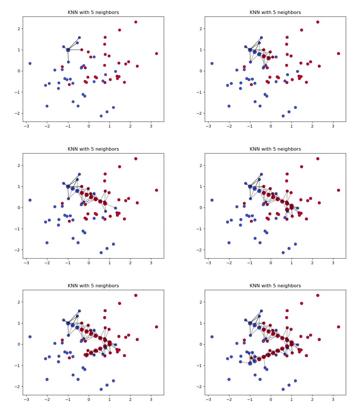
NOTE: all figures in this post were made by the author using \(\LaTeX\),
numpy, andmatplotlib
We use distance formulas in \(k\)-NN to determine the proximity of data points in order to make predictions or classifications based on the neighbors. There are many ways to measure similarity, along with many instances where one formula should be used over another.
Euclidean Distance
The first—and most common—distance formula is the Euclidean distance.
This is calculated by finding the difference between elements in list \(x\) with elements in list \(y\), calculating the sum of those differences, and taking the square root of the sum. This finds the linear distance between two points.
Euclidean distance is a straightforward measure of spatial similarity, making it suitable for many applications. It is used when the features have a clear geometric interpretation, and scale differences between features are not a concern as scale difference is a major drawback with this metric.
Manhattan Distance
This distance formula is different from Euclidean distance because it does not measure the magnitude nor the angle of the line connecting two points. In certain instances, knowing the magnitude of the line between two points is necessary in a \(k\)-NN problem.
When classifying a point, a shorter distance between that point and another point of a different class often indicates a higher similarity between the points. Consequently, the point is more likely to belong to the class that is closer to it.
You can see the difference in Euclidean distance and Manhattan distance more clearly in the image below. The formula on the right resembles the distance from one street to another in a city grid, hence the name “Manhattan” distance.
The Manhattan distance can be particularly useful in datasets or scenarios where the features have different units of measurement that are all independent of each other. It captures the total discrepancy along each feature dimension without assuming any specific relationship between them.
When calculating the similarity or distance between two houses, using the Euclidean distance would implicitly assume that the features contribute equally to the overall similarity with a straight line connecting them. However, in reality, the differences in square footage, distance to a local school, number of bedrooms, etc. might not have equal importance.
Minkowski Distance
This distance formula is unique in that it includes both Euclidean and Manhattan distances as special cases, when \(p=2\) and \(p=1\), respectively. Using this distance formula allows us to control a single variable, \(p\), to get either formula.
Note that sklearn.neighbors.KNeighborsClassifier() function uses Minkowski distance as the default metric, most likely because of its versatility. Refer to scipy.spatial.distance() for a complete list of distance metrics.
In general, a higher value of \(p\) can give more importance to larger differences between feature values, while a lower value of \(p\) can prioritize individual feature differences.
Cosine Similarity
If you’ve taken a linear algebra class, you’ve definitely seen this formula before. This equation calculates \(\cos{(\theta)}\), where \(\theta\) represents the angle between two non-zero feature vectors. It involves taking the dot product of two vectors in the numerator, then dividing it by the length of each vector.
In a linear algebra textbook, you might see a similar equation that looks like this:
This is the same formula, where \(\vec{x}\) and \(\vec{y}\) represent two feature vectors, and \(||\vec{x}||\) and \(||\vec{y}||\) are the lengths of each vector. This formula measures the similarity of two vectors, and it is helpful to remember that the range of cosine is between \(-1\) and \(1\). Vectors where \(\cos{(\theta)} \approxeq -1\), have exact dissimilarity, \(\cos{(\theta)} \approxeq 0\) (orthogonal vectors if you know your linear algebra), have no similarity, and \(\cos{(\theta)} \approxeq 1\) have the exact similarity. This can be seen graphically, as below:
In the example above, the cosine similarity between the two vectors is \(-0.7642\), which indicates \(\vec{x}\) and \(\vec{y}\) are have a strong degree of dissimilarity.
You can see the differences in each of the three cosine similarities below. In the leftmost graph, since the two vectors are perpendicular, they have no similarity.
In the middle graph, since the two vectors are multiples of each other, and they have the same direction, they fall on the same line in 2D space. This means they are essentially the same vector—exact similarity—just with a different magnitude. This is apparent because we have \(2\vec{x} = \vec{y}\) in the middle graph.
Finally, in the rightmost graph, these two vectors are exactly dissimilar, with a similarity of \(-1\). Like in the middle graph, these vectors are indeed multiples of each other since we have \(-1\vec{x} = \vec{y}\). The key difference here is that the negative magnitude changes the direction of \(\vec{y}\) to the exact opposite of \(\vec{x}\).
Hamming Distance
If we wanted to classify a binary output, this is the metric we want to use. The function \(\delta\) is the Kronecker delta function, which returns \(1\), or True if \(x_i = y_i\), and \(0\), or False if \(x_i \neq y_i\). It measures the number of positions at which two vectors differ. It is commonly used in various fields, including biology, for comparing sequences such as DNA molecules to identify the positions where they differ.
